Following on the tails of demographic research and land cover research manuscripts, UHPSI recently completed a new manuscript focused on thematic map accuracy assessment.
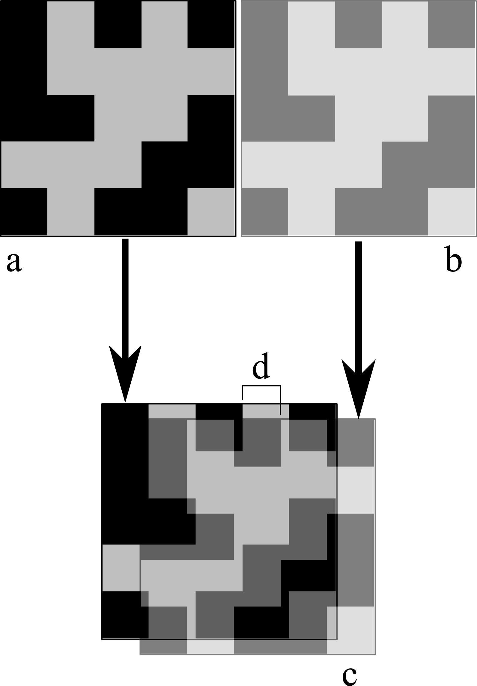
Co-registration error between mapped locations. (a) represents locations derived from GPS technology; (b) represents locations derived from aerial or satellite imagery; (c) represents the accuracy assessment process where the two must be co-registered for comparison; (d) represents the coregistration error distance, or how much the representations are misaligned.
The nature of scientific research is that while investigating one’s primary area of inquiry one inevitably stumbles upon new ideas. An example of this came as we began the accuracy assessment of a high spatial resolution categorical map of the Ucross Ranch. During the assessment process we began to question some of the most common metrics used to quantify accuracy, and so designed a custom computer program to perform a series of tests that evaluate the utility of these metrics. The basic concept we explored had to do with co-registration, which we’ll explain.
As illustrated in the figure to the right, mapping relies on two digital conceptualizations of where things are in space, each of which has its own sources of error. One conceptualization (inset a) is derived from GPS technology, which can tell us where on the globe we are using a constellation of satellites. When you are out in the field with a GPS unit, you know exactly where you are, since you’re standing right there. The GPS unit is there to provide you with a numerical version of your experience (i.e. coordinates). The GPS location of a given place in the world, for instance, the upper lefthand black pixel in a, is represented mathematically using a central measuring station (called a datum), a generalized model of the Earth’s shape (called a geoide), and algorithms that triangulate position, among other things. Because the satellites are so far away, because they are traveling at such high speeds, and because generalized models are used, our numerical estimates of our locations are subject to error. When we present a series of GPS points in space — the entire lefthand pixelated image — we do the best we can but recognize that the locations might not be perfectly correct with respect to their “true” locations.
A second form of error comes when trying to create a two-dimensional image or map of the Earth’s three-dimensional surface, represented by the righthand pixelated inset b. Here we apply transformation functions that convert the geographic coordinates of a given location to visually appealing locations on a flat surface. There are lots of transformation functions (called projections), many of which preserve specific facets of real-world attributes. For instance, some two dimensional maps preserve the area of mapped units while others preserve linear distance. Between the 3D to 2D conversion and the Earth’s topographic relief, images we take from planes and satellites, or maps we produce using those technologies, have some inherent degree of error.
Now, to properly assess the accuracy of a map of the Ucross Ranch, we had to compare “true” locations obtained using GPS with mapped locations derived from an image (inset c). Because of the inherent errors in the GPS and mapped predictions, we inevitably end up with co-registration error when we represent them numerically or digitally on a computer. That is, the two don’t line up properly, as shown in inset c. The amount that they are misaligned, labed “d” for distance, is usually unknown, and as scientists we don’t know what effect co-registration error has on the estimated accuracy of our maps. In our study however, we were able to determine how accuracy changes as co-registration error increases. This allowed us to build mathematical models that let us predict, which good precision, how two measures of accuracy changed with increasing co-registration error. This also allowed us to invert our models to determine how much co-registration error we had in our initial accuracy assessment, and how much it artificially lowered our estimates of accuracy.
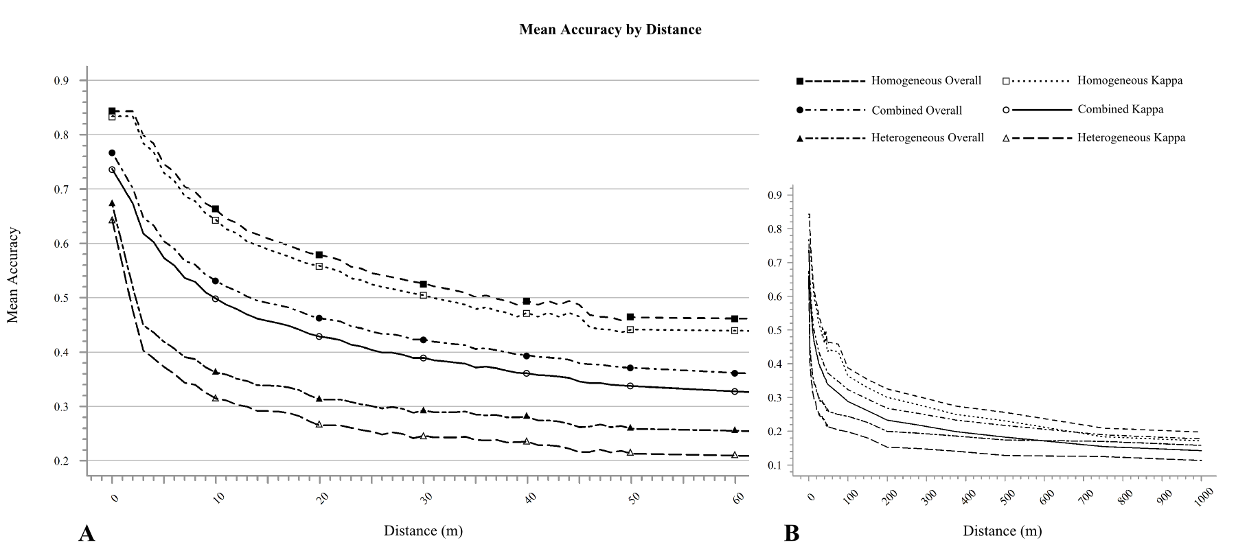
The results of Monte Carlo simulations in which co-registration error was sequentially increased to greater and greater distances. The plots show the mean values for two types of accuracy, overall accuracy and Cohen’s kappa coefficient, when simulated 100 times at each distance (on the x axis). Each set of two accuracy curves corresponds to a different core dataset. The plots are the same with the exception that A shows only distances 0-60 m of horistonal displacement between images and B shows 0-1000m.